Measuring Goodhart’s Law

Measuring Goodhart’s Law?

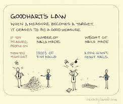
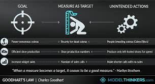
According to the famous Goodhart’s law, “a measure ceases to be a good measure when it becomes a target.” Although it comes from economics, we at OpenAI have to consider it when deciding how to optimise goals that are challenging or expensive to quantify. It is frequently important to incorporate a proxy objective that is simpler or less expensive to measure, but we must be careful not to overoptimize it.

For instance, we would like to optimise questions like “How helpful is this response?” or “How factually correct is this claim?” as part of our efforts to match models like GPT-3 with human intent and values. These are intricate goals that call for meticulous human inspection. For this reason, we develop a reward model that can forecast these preferences in humans and utilise its predictions as a stand-in objective. Nonetheless, it’s crucial to monitor how well the real objective is optimised.

We’ll examine some of the mathematics underlying how we achieve this in this piece. We’ll concentrate on a situation that is easy to examine and where we can see the real goal. In reality, even our preferences sometimes fall short of capturing what matters to us most, but we’ll ignore that problem for the purposes of this essay.

Best-of-n sampling

There are various techniques to improve the proxy objective, but best-of-n sampling, also known as rejection sampling or reranking, is perhaps the simplest. Simply, we take the sample with the greatest proxy objective score out of n samples.

Even though it requires more inference-time computation, this strategy can really compete with more sophisticated approaches like reinforcement learning. In WebGPT, for instance, our best-of-64 64 model fared better than our reinforcement learning model, maybe in part because it had access to a larger number of websites. Even using best-of-four-four gave human preferences a notable boost.

Also, best-of-n sampling performs consistently and is simple to quantitatively analyse, making it a good choice for empirical research of Goodhart’s law and associated phenomena.

The mathematics of best-of-n sampling

Let’s conduct a more rigorous investigation of best-of-n sampling. Assume we have a real aim (or “reward”) true, some probability distribution P over S, and some sample space S (like the set of potential question-answer pairs): R true: SR, and R proxy: SR for an objective proxy. Let’s imagine we manage to improve proxy R proxy and get a new distribution P ′ as a result. Then:

The assumption is that [true (′)] E x ′ P ′ [R true (x ′)] evaluates how well the true goal has been optimised.

How successfully we have optimised the genuine objective is indicated by the value of [R true (x ′)].

KL’s divergence We can measure how much optimization we have done using KL (′ ) D KL (P ′ P). This KL divergence is just the negative log probability that a sample from P lies in ′ S ′, for instance, if ′ P ′ is created by picking the first sample from P that lies in some subset ′ S ′ S.

It turns out that both of these values can be accurately approximated using samples from P in the case of best-of-n sampling.

Let’s start by examining the expectation. Using a Monte Carlo estimator is the naive method, which entails performing best-of-n sampling repeatedly, measuring the true goal on those samples, and averaging the outcomes. There is, however, a superior estimator. If we have N n samples from P overall, we can simultaneously consider every conceivable subset of these samples of size n, weight each sample by the quantity of subgroups for which it is the best in terms of the proxy objective, and then calculate the weighted average true objective score. This weight is essentially the binomial coefficient ( 1 1 ) ( n k ) from 1 1 where k is the rank of the sample under the proxy objective. to the worst of N (best). [1] In addition to making better use of samples, this enables us to reuse samples for various n values.

Surprisingly, the KL divergence has a precise formula that applies to any continuous probability distribution P (i.e., as long as P has no point masses). As best-of-n essentially involves taking the to1 n 1 of the distribution, one may naively assume that the solution is log login. This assumption is roughly accurate, however the precise solution is log 1 1 login n n1. [2]

When used together, these estimators make it simple to examine how the underlying objective changes depending on how much optimization is done to the proxy objective.

Here’s a real-life example from WebGPT:

Best-of-n performance for WebGPT 175B

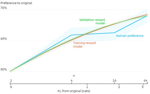
Performance for WebGPT using the best-of-n method, with shaded areas denoting 11 standard error and the KL axis using a square root scale. Here, the training reward model, a validation reward model trained on held-out data, and actual human preferences are considered as three putatively “true” objectives (true R true). The training reward model itself, a validation reward model, and the original distribution (P) are all given by the 175B model trained using behaviour cloning. The proxy target is not overly optimised much, but at higher KLs, we would anticipate it to be.

Going beyond best-of-n sampling

The fundamental drawback of best-of-n sampling is that it can only be used sparingly for optimization because the KL divergence grows logarithmically with n.

Reinforcement learning is often used to apply more optimization. We’ve often been able to use reinforcement learning to achieve a KL of approximately 10 nats in the scenarios we’ve explored thus far, like summarization, before Goodhart’s rule causes the real aim to begin to decline. To achieve this KL using best-of-n, n would need to be roughly 60,000, but we anticipate being able to achieve considerably higher KLs using improved reward modelling and reinforcement learning techniques.

Yet not all nats are created equal. Empirically, best-of-n outperforms reinforcement learning in optimising the real and proxy objectives for modest KL budgets. Best-of-n is the “brute force” method, and as such, it is less computationally efficient for large KLs but more information theoretically efficient than reinforcement learning.

© 2023. All Rights Reserved. Designed by Animesh Mogha